The mpatrol library has the capability to summarise the information it accumulated about the behaviour of dynamic memory allocations and deallocations over the lifetime of any program that it was linked and run with. This summary shows a rough profile of all memory allocations that were made, and is hence called profiling. There are several other different kinds of profiling provided with most compilation tools, but they generally profile function calls or line numbers in combination with the time it takes to execute them.
Memory allocation profiling is useful since it allows a programmer to see which functions directly allocate memory from the heap, with a view to optimising the memory usage or performance of a program. It also summarises any unfreed memory allocations that were present at the end of program execution, some of which could be as a result of memory leaks. In addition, a summary of the sizes and distribution of all memory allocations and deallocations is available.
A memory allocation call graph is also available for the programmer to be able to see the caller and callee relationships for all functions that allocated memory, either directly or indirectly. This graph is shown in a tabular form similar to that of gprof, but it can also be written to a graph specification file for later processing by dot. The dot and dotty commands are part of GraphViz, an excellent graph visualisation package that was developed at AT&T Bell Labs and is available for free download for UNIX and Windows platforms from http://www.research.att.com/sw/tools/graphviz/.
Only allocations and deallocations are recorded, with each reallocation being treated as a deallocation immediately followed by an allocation. For full memory allocation profiling support, call stack traversal must be supported in the mpatrol library and all of the program's symbols must have been successfully read by the mpatrol library before the program was run. The library will attempt to compensate if either of these requirements are not met, but the displayed tables may contain less meaningful information. Cycles that appear in the allocation call graph are due to recursion and are currently dealt with by only recording the memory allocations once along the call stack.
Memory allocation profiling is disabled by default, but can be enabled using the PROF option. This writes all of the profiling data to a file called mpatrol.out in the current directory at the end of program execution, but the name of this file can be changed using the PROFFILE option and the default directory in which to place these files can be changed by setting the PROFDIR environment variable. Sometimes it can also be desirable for the mpatrol library to write out the accumulated profiling information in the middle of program execution rather than just at the end, even if it is only partially complete, and this behaviour can be controlled with the AUTOSAVE option. This can be particularly useful when running the program from within a debugger, when it is necessary to analyse the profiling information at a certain point during program execution.
When profiling memory allocations, it is necessary to distinguish between small, medium, large and extra large memory allocations that were made by a function. The boundaries which distinguish between these allocation sizes can be controlled via the SMALLBOUND, MEDIUMBOUND and LARGEBOUND options, but they default to 32, 256 and 2048 bytes respectively, which should suffice for most circumstances.
The mprof command is a tool designed to read a profiling output file produced by the mpatrol library and display the profiling information that was obtained. The profiling information includes summaries of all of the memory allocations listed by size and the function that allocated them and a list of memory leaks with the call stack of the allocating function. It also includes a graph of all memory allocations listed in tabular form, and an optional graph specification file for later processing by the dot graph visualisation package.
The mprof command also attempts to calculate the endianness of the processor that produced the profiling output file and reads the file accordingly. This means that it is possible to use mprof on a SPARC machine to read a profiling output file that was produced on an Intel 80x86 machine, for example. However, this will only work if the processor that produced the profiling output file has the same word size as the processor that is running the mprof command. For example, reading a 64-bit profiling output file on a 32-bit machine will not work.
In addition, the profiling output file also contains the version number of the mpatrol library which produced it. If the major version number that is embedded in the profiling output file is newer that the version of mpatrol that mprof came with then mprof will refuse to read the file. You should download the latest version of mpatrol in that case. The reason for storing the version number is so that the format of the profiling output file can change between releases of mpatrol, but also allow mprof to cope with older versions.
Along with the options listed below, the mprof command takes one optional argument which must be a valid mpatrol profiling output filename but if it is omitted then it will use mpatrol.out as the name of the file to use. If the filename argument is given as `-' then the standard input file stream will be used as the profiling output file. Note also that the mprof command supports the --help and --version options in common with the other mpatrol command line tools.
We'll now look at an example of using the mpatrol library to profile the dynamic memory allocations in a program. However, remember that this example will only fully work on your machine if the mpatrol library supports call stack traversal and reading symbols from executable files on that platform. If that is not the case then only some of the features will be available.
The following example program performs some simple calculations and displays a list of numbers on its standard output file stream, but it serves to illustrate all of the different features of memory allocation profiling that mpatrol is capable of. The source for the program can be found in tests/profile/test1.c.
     23  /*
     24   * Associates an integer value with its negative string equivalent in a
     25   * structure, and then allocates 256 such pairs randomly, displays them
     26   * then frees them.
     27   */


     30  #include <stdio.h>
     31  #include <stdlib.h>
     32  #include <string.h>


     35  typedef struct pair
     36  {
     37      int value;
     38      char *string;
     39  }
     40  pair;


     43  pair *new_pair(int n)
     44  {
     45      static char s[16];
     46      pair *p;

     48      if ((p = (pair *) malloc(sizeof(pair))) == NULL)
     49      {
     50          fputs("Out of memory\n", stderr);
     51          exit(EXIT_FAILURE);
     52      }
     53      p->value = n;
     54      sprintf(s, "%d", -n);
     55      if ((p->string = strdup(s)) == NULL)
     56      {
     57          fputs("Out of memory\n", stderr);
     58          exit(EXIT_FAILURE);
     59      }
     60      return p;
     61  }


     64  int main(void)
     65  {
     66      pair *a[256];
     67      int i, n;

     69      for (i = 0; i < 256; i++)
     70      {
     71          n = (int) ((rand() * 256.0) / (RAND_MAX + 1.0)) - 128;
     72          a[i] = new_pair(n);
     73      }
     74      for (i = 0; i < 256; i++)
     75          printf("%3d: %4d -> \"%s\"\n", i, a[i]->value, a[i]->string);
     76      for (i = 0; i < 256; i++)
     77          free(a[i]);
     78      return EXIT_SUCCESS;
     79  }
After the above program has been compiled and linked with the mpatrol library, it should be run with the PROF option set in the MPATROL_OPTIONS environment variable. Note that mpatrol.h was not included as it is not necessary for profiling purposes.
If all went well, a list of numbers should be displayed on the screen and a file called mpatrol.out should have been produced in the current directory. This is a binary file containing the total amount of profiling information that the mpatrol library gathered while the program was running, but it contains concise numerical data rather than human-readable data. To make use of this file, the mprof command must be run. An excerpt from the output produced when running mprof with the --call-graph option is shown below1.
                                  ALLOCATION BINS

                               (number of bins: 1024)

                       allocated                          unfreed
            --------------------------------  --------------------------------
      size   count       %     bytes       %   count       %     bytes       %

         2       9    1.76        18    0.61       9    3.52        18    1.95
         3     105   20.51       315   10.61     105   41.02       315   34.16
         4     121   23.63       484   16.30     121   47.27       484   52.49
         5      21    4.10       105    3.54      21    8.20       105   11.39
         8     256   50.00      2048   68.96       0    0.00         0    0.00

     total     512              2970             256               922
                                 DIRECT ALLOCATIONS

                      (0 < s <= 32 < m <= 256 < l <= 2048 < x)

            allocated                       unfreed
     --------------------------  --------------------------
     bytes       %   s  m  l  x  bytes       %   s  m  l  x  count  function

      2970  100.00  %%             922  100.00  %%             512  new_pair

      2970          %%             922          %%             512  total
                                    MEMORY LEAKS

                              (maximum stack depth: 1)

                     unfreed                      allocated
     ----------------------------------------  ----------------
          %     bytes       %   count       %     bytes   count  function

     100.00       922   31.04     256   50.00      2970     512  new_pair

                  922   31.04     256   50.00      2970     512  total
                               ALLOCATION CALL GRAPH

                              (number of vertices: 3)

                allocated               unfreed
          ---------------------  ---------------------
     index   bytes   s  m  l  x     bytes   s  m  l  x  function
     -------------------------------------------------
     [1]                                                _start [1]
              2970  %%                922  %%               main [3]
     -------------------------------------------------
              2970  %%                922  %%               main [3]
     [2]                                                new_pair [2]
     -------------------------------------------------
              2970  %%                922  %%               _start [1]
     [3]                                                main [3]
              2970  %%                922  %%               new_pair [2]
The first table shown is the allocation bin table which summarises the sizes of all objects that were dynamically allocated throughout the lifetime of the program. In this particular case, counts of all allocations and deallocations of sizes 1 to 1023 bytes were recorded by the mpatrol library in their own specific bin and this information was written to the profiling output file. Allocations and deallocations of sizes larger than or equal to 1024 bytes are counted as well and the total number of bytes that they represent are also recorded. This information can be extremely useful in understanding which sizes of data structures are allocated most during program execution, and where changes might be made to make more efficient use of the dynamically allocated memory.
As can be seen from the allocation bin table, 9 allocations of 2 bytes, 105 allocations of 3 bytes, 121 allocations of 4 bytes, 21 allocations of 5 bytes and 256 allocations of 8 bytes were made during the execution of the program. However, all of these memory allocations except the 8 byte allocations were still not freed by the time the program terminated, resulting in a total memory leak of 922 bytes.
The next table shown is the direct allocation table which lists all of the functions that allocated memory and how much memory they allocated. The `s m l x' columns represent small, medium, large and extra large memory allocations, which in this case are 0 bytes is less than a small allocation, which is less than or equal to 32 bytes, which is less than a medium allocation, which is less than or equal to 256 bytes, which is less than a large allocation, which is less than or equal to 2048 bytes, which is less than an extra large allocation. The numbers listed under these columns represent a percentage of the overall total and are listed as `%%' if the percentage is 100% or as `.' if the percentage is less than 1%. Percentages of 0% are not displayed.
The information displayed in the direct allocation table is useful for seeing
exactly which functions in a program directly perform memory allocation, and can
quickly highlight where optimisations can be made or where functions might be
making unnecessary allocations. In the example, this table shows us that 2970
bytes were allocated over 512 calls by new_pair() and that 922 bytes were
left unfreed at program termination. All of the allocations that were made by
new_pair() were between 1 and 32 bytes in size.
We could now choose to sort the direct allocation table by the number of calls
to allocate memory, rather than the number of bytes allocated, with the
--counts option to mprof, but that is not relevant in this
example. However, we know that there are two calls to allocate memory from
new_pair(), so we can use the --addresses option to
mprof to show all call sites within functions rather than just the
total for each function. This option does not affect the allocation bin table
so the new output from mprof with the --call-graph and
--addresses options looks like:
                                 DIRECT ALLOCATIONS

                      (0 < s <= 32 < m <= 256 < l <= 2048 < x)

            allocated                       unfreed
     --------------------------  --------------------------
     bytes       %   s  m  l  x  bytes       %   s  m  l  x  count  function

      2048   68.96  69               0    0.00                 256  new_pair+20
       922   31.04  31             922  100.00  %%             256  new_pair+140

      2970          %%             922          %%             512  total
                                    MEMORY LEAKS

                              (maximum stack depth: 1)

                     unfreed                      allocated
     ----------------------------------------  ----------------
          %     bytes       %   count       %     bytes   count  function

     100.00       922  100.00     256  100.00       922     256  new_pair+140

                  922   31.04     256   50.00      2970     512  total
                               ALLOCATION CALL GRAPH

                              (number of vertices: 4)

                allocated               unfreed
          ---------------------  ---------------------
     index   bytes   s  m  l  x     bytes   s  m  l  x  function
     -------------------------------------------------
     [1]                                                _start+100 [1]
              2970  %%                922  %%               main+120 [4]
     -------------------------------------------------
              2048  %%                  0                   main+120 [4]
     [2]                                                new_pair+20 [2]
     -------------------------------------------------
               922  %%                922  %%               main+120 [4]
     [3]                                                new_pair+140 [3]
     -------------------------------------------------
              2970  %%                922  %%               _start+100 [1]
     [4]                                                main+120 [4]
              2048  %%                  0                   new_pair+20 [2]
               922  %%                922  %%               new_pair+140 [3]
The names of the functions displayed in the above tables now have a byte offset
appended to them to indicate at what position in the function a call to allocate
memory occurred2. Now it is possible to see that the first call to allocate memory
from within new_pair() has had all of its memory freed, but the second
call (from strdup()) has had none of its memory freed.
This is also visible in the next table, which is the memory leak table and lists all of the functions that allocated memory but did not free all of their memory during the lifetime of the program. The default behaviour of mprof is to show only the function that directly allocated the memory in the memory leak table, but this can be changed with the --stack-depth option. This accepts an argument specifying the maximum number of functions to display in one call stack, with zero indicating that all functions in a call stack should be displayed. This can be useful for tracing down the functions that were indirectly responsible for the memory leak. The new memory leak table displayed by mprof with the --addresses and --stack-depth 0 options looks like:
                                    MEMORY LEAKS

                              (maximum stack depth: 0)

                     unfreed                      allocated
     ----------------------------------------  ----------------
          %     bytes       %   count       %     bytes   count  function

     100.00       922  100.00     256  100.00       922     256  new_pair+140
                                                                 main+120
                                                                 _start+100

                  922   31.04     256   50.00      2970     512  total
Now that we know where the memory leak is coming from, we can fix it by freeing the string as well as the structure at line 77. A version of the above program that does not contain the memory leak can be found in tests/profile/test2.c.
The final table that is displayed is the allocation call graph, which shows the
relationship between a particular function in the call graph, the functions that
called it (parents), and the functions that it called (children). Every
function that appears in the allocation call graph is displayed with a
particular index that can be used to cross-reference it. The functions which
called a particular function are displayed directly above it, while the
functions that the function called are displayed directly below it. In the
above example, _start() called main(), which then called
new_pair() which allocated the memory.
The memory that has been allocated by a function (either directly, or indirectly by its children) for its parents is shown in the details for the parent functions, showing both a breakdown of the allocated memory and a breakdown of the unfreed memory. This also occurs for the child functions. If a function does not directly allocate memory then the total memory allocated for its parents will equal the total memory allocated by its children. However, if a parent or child function is part of a cycle in the call graph then a `(*)' will appear in the leftmost column of the call graph. In that case the total incoming memory may not necessarily equal the total outgoing memory for the main function.
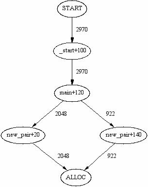
In the example above when the --addresses option is used, it should be
clear that new_pair()+20 allocates 2048 bytes for main(), while
new_pair()+140 allocates 922 bytes for main(). The main()
function itself allocates 2970 bytes for _start() overall via the
new_pair() function.
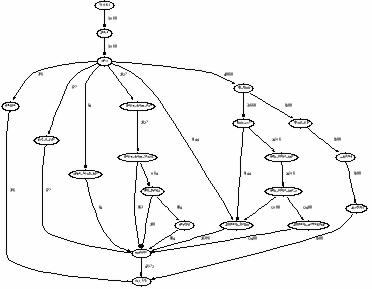
It is also possible to view this information graphically if you have the GraphViz package mentioned above installed on your system. The --graph-file option can be used to write a dot graph specification file that can be processed by the dot or dotty commands that come with GraphViz. The resulting graphs will show the relationships between each function, its parents and its children, and will also show the number of bytes that were allocated along the edges of the call graph, but this can be changed to the number of calls if the --counts option is used3. A call graph showing unfreed memory instead of allocated memory can be generated by adding the --leaks option. The following graph illustrates the use of these options with the above example. It was generated using the --addresses and --graph-file options.
As a final demonstration of mpatrol's profiling features we will attempt to profile a real application in order to see where the memory allocations come from. Since all of the following steps were performed on a Solaris machine, the --dynamic option of the mpatrol command was used to allow us to replace the system memory allocation routines with mpatrol's routines without requiring a relink. It also means that we can profile all of the child processes that were created by the application as well.
The application that we are going to profile is the GNU C compiler, gcc (version 2.95.2), which is quite a complicated and large program. The actual gcc command is really the compiler driver which invokes the C preprocessor followed by the compiler, the assembler, the prelinker and finally the linker (well, it does in this example). On Solaris, the gcc distribution uses the system assembler and linker which come with no symbol tables in their executable files so we will not be profiling them.
For the purpose of this demonstration we will only be looking at the graph files produced by the --graph-file option of the mprof command, but ordinarily you would want to look at the tables that mprof produces as well. All of the command line examples use the bash shell but in most cases these will work in other shells with a minimal amount of changes.
We will use tests/profile/test2.c as the source file to compile with gcc and we'll turn on optimisation in order to cause gcc to allocate a bit more memory than it would normally. Note that use is also made of the format string feature of the --log-file and --prof-file options so that it is clear which mpatrol log and profiling output files belong to which processes.
     bash$ mpatrol --dynamic --log-file=%p.log --prof-file=%p.out
                   --prof gcc -O -o test2 test2.c
     bash$ ls *.log *.out
     as.log         cc1.out        cpp.log        gcc.out
     as.out         collect2.log   cpp.out        ld.log
     cc1.log        collect2.out   gcc.log        ld.out
As mentioned above, we're not interested in the mpatrol log and profiling output files for as and ld so we'll delete them. We can now use mprof to create graph specification files for each of the profiling output files produced. You can find these graph specification files and the profiling output files used to generate them in the extra directory in the mpatrol distribution.
     bash$ rm as.log as.out ld.log ld.out
     bash$ ls *.out
     cc1.out        collect2.out   cpp.out        gcc.out
     bash$ for file in *.out
     > do
     >     mprof --graph-file=`basename $file .out`.dot $file
     > done >/dev/null
     bash$ ls *.dot
     cc1.dot        collect2.dot   cpp.dot        gcc.dot
The graph specification files that have now been produced can be viewed and manipulated with the dotty command, or they can be converted to various image formats with the dot command. However, this presumes that you already have the GraphViz graph visualisation package installed. If you have then you can convert the graph specification files to GIF and postscript images using the following commands. If not, you can still view the graphs produced in the following figures.
     bash$ dot -Tgif -Gsize="6,3" -Gratio=fill -o gcc.gif gcc.dot
     bash$ dot -Tgif -Gsize="6,3" -Gratio=fill -o cpp.gif cpp.dot
     bash$ dot -Tgif -Gsize="7,4" -Gratio=fill -o cc1.gif cc1.dot
     bash$ dot -Tgif -Gsize="4,3" -Gratio=fill -o collect2.gif collect2.dot
     bash$ dot -Tps -Gsize="6,3" -Gratio=fill -o gcc.ps gcc.dot
     bash$ dot -Tps -Gsize="6,3" -Gratio=fill -o cpp.ps cpp.dot
     bash$ dot -Tps -Gsize="9,6" -Gratio=fill -Grotate=90 -o cc1.ps cc1.dot
     bash$ dot -Tps -Gsize="4,3" -Gratio=fill -o collect2.ps collect2.dot
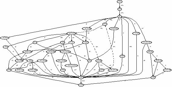
The figure above shows the allocation call graph for the gcc compiler
driver. From the graph you can see that the vast majority of memory allocations
appear to be required for reading the driver specification file, which details
default options and platform-specific features. Almost all of the memory
allocations go through the xmalloc() routine, which is an error-checking
function built on top of malloc()4. A large amount of memory is also allocated by
the obstack module, which provides a functionality similar to
arenas for variable-sized data structures. You'll see extensive use of
both of these types of routines throughout the following graphs.
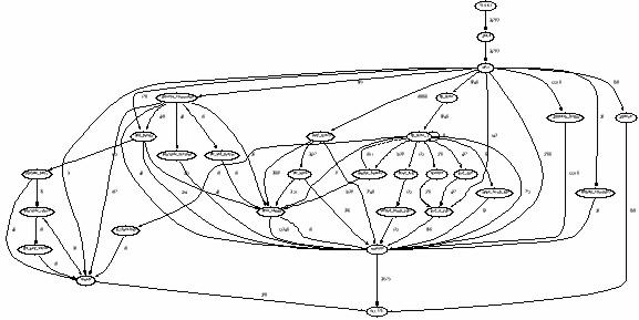
As would be expected, in the above allocation call graph for the cpp
C preprocessor, the majority of memory allocations are used for macro
processing, with a sizable chunk being allocated for reading include files.
You may also notice the dotted lines that connect the rescan(),
handle_directive(), do_include() and finclude()
functions5. These
show a cycle in the call graph where each of these functions may have been
involved in one or more recursive calls. The labels for such dotted edges may
not be entirely accurate since mprof will only count allocated memory
once for each recursive call chain.
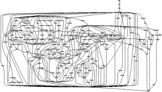
The following figure shows the allocation call graph for the cc1
compiler itself. As you would expect, it's a bit of a beast compared to the
previous two graphs, and looks very hard to follow. However, if you look closer
you will notice that the various groups of functions that comprise the compiler
stand out due to their close association with one another. For example, you
might notice that the functions between cse_insn() and
get_cse_reg_info() form a group that allocates 9140 bytes overall. You
can also see the parser module at the top left of the graph, initiated with
yyparse(), and the code generator module in the rest of the graph,
initiated with rest_of_compilation().
The allocation call graph for the prelinker, collect2, is a lot
simpler than the previous graphs. There are no cycles in the graph and most of
the allocations are concerned with maintaining hash tables. Once again,
xmalloc() and _obstack_begin() are the two main sources of memory
allocation.
As can be seen, a lot of information about the memory allocation behaviour of a program can be obtained by creating a visual image of the allocation call graph. In addition, different graphs can be produced to show call counts instead of allocated bytes (via the --counts option), and graphs of unfreed memory can be produced to detect where memory leaks come from (via the --leaks option).
Although mprof does not currently offer this facility, a small tool called profdiff which reports differences between two mpatrol profiling output files can be downloaded from http://heanet.dl.sourceforge.net/sourceforge/mpatrol/mpatrol_patch3.tar.gz.
Much of the functionality of this implementation of memory allocation profiling is based upon mprof by Benjamin Zorn and Paul Hilfinger, which was written as a research project and ran on MIPS, SPARC and VAX machines. However, the profiling output files are incompatible, the tables displayed have a different format, and the way they are implemented is entirely different.
[1] The --call-graph option is only needed to display the allocation call graph table, which is not normally displayed by default.
[2] If no symbols could be read from the program's executable file, or if the corresponding symbol could not be determined, then the function names will be replaced with the code addresses at which the calls took place.
[3] Cycles in the graph are marked by dashed lines along the relevant edges instead of solid lines.
[4] The mpatrol version of
xmalloc() was not used in this case since another version of
xmalloc() was originally statically linked into the program being run,
and so could not be overridden.
[5] You might also have noticed the dotted lines connecting
do_spec_1() and handle_braces() in the previous graph.